Invertible fixed-point complex rotation
Geraint Luff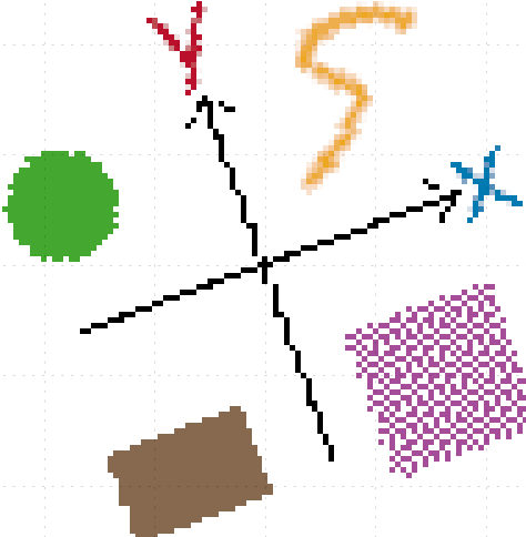
A look at how to perform lossless rotations on integer / fixed-point co-ordinates or complex values.
This is a slightly longer one - sorry about that! The first half lays out some cool ideas, and then we have to deal with some of the things we glossed over.
The problem
Let's say you have a integer (or fixed-point) complex value, and you want to perform a complex rotation:

The problem is that the result doesn't lie exactly on one of the fixed-point values. There are a couple of obvious ways to handle this:
- Use a larger fixed-point data format for the result, treating the extra bits as fractional.
- Round the result to the nearest fixed-point value
The problem with a larger data-type is that... well, now you're computing and storing a larger data-type. But in fact, both of these solutions run into trouble with invertibility.
Invertibility
If you add two fixed-point complex numbers together, you can subtract them again, to (perfectly) get your original answer back. Even integer overflows don't actually screw up this property.
It would be great to have the same property for our rotation: if we take our rotated result and perform the opposite rotation, we should get our original point back.
Simple rounding (our second approach above) fails on this because two different input values might round to the same result when rotated. If that happens, how can the inverse rotation know which one to return?
What do we need?
If we want our rotation to be perfectly invertible, and not need a larger data-type, then every possible value on our grid has to map to a distinct point on the same grid. If we have
Let's take a little detour into a related problem:
Detour: losslessly rotating an image
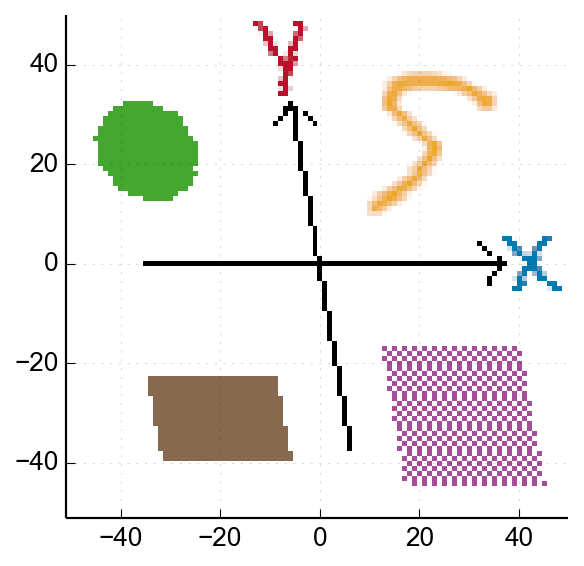
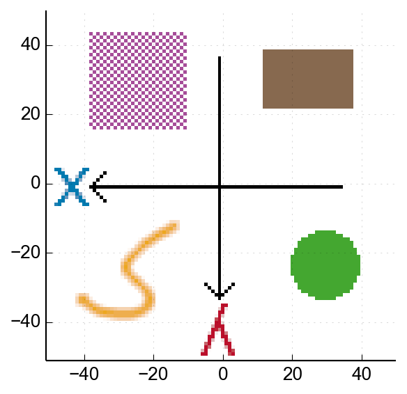
Let's say we have a 100x100 pixel image:
Let's say we want to rotate this image, but with no interpolation, or dropping/duplicating pixels. The result should be the same size, but we don't mind a bit of wrapping-around at the edges. This means that all we're doing is shuffling pixels around inside the image.
This image rotation is equivalent to our complex-rotation problem. Each fixed-point complex number can be considered as a pixel co-ordinate within the image, which is then be mapped to a new (rotated) position.
Skewing the image
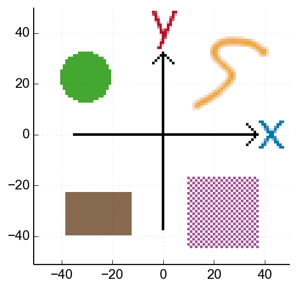
One operation we can definitely do losslessly is skewing. Here's a horizontal skew, where each row in the image is shifted horizontally by 15% of its vertical position:
This corresponds to the matrix:
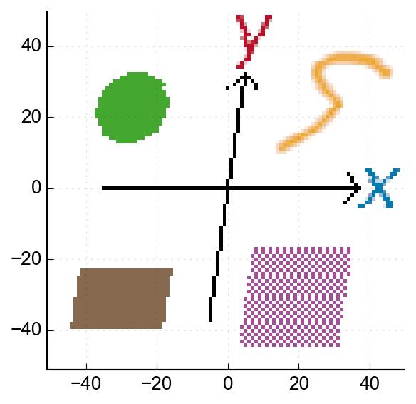
Since all we've done is shift rows around, it's entirely reversible - if you applied the opposite skew to that result above, you would restore the original image.
Here's a -25% vertical skew, corresponding to the matrix:
Approximating a rotation
What we actually want is this rotation matrix:
If we can express this matrix as the product of skew matrices (corresponding to a sequence of skew operations), then each pixel will end up approximately in its rotated position. It's approximate because we have to round the co-ordinates after every step.
It turns out we need three steps to make this work. If we define
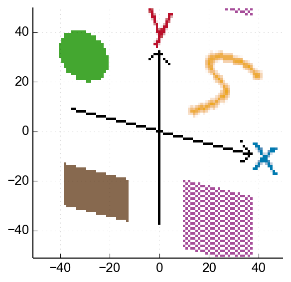
This corresponds to a horizontal skew, a vertical skew, and another horizontal skew:
➔
 ➔
➔
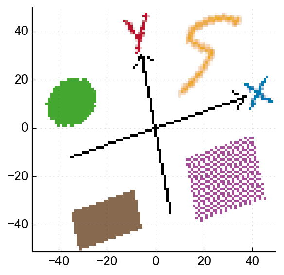 ➔
➔
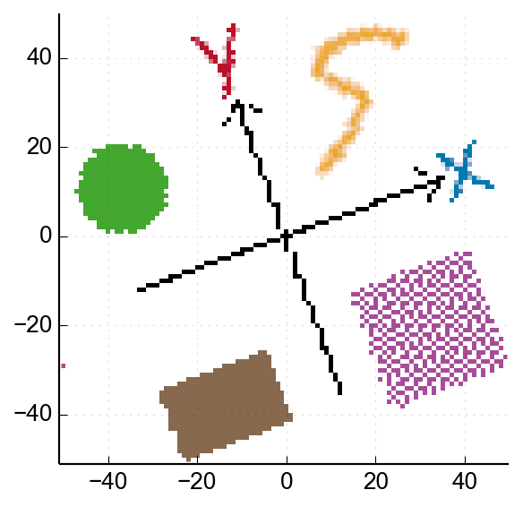
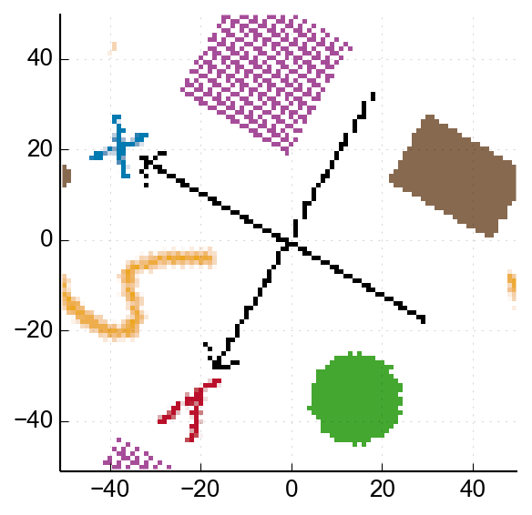
The result is a rotated version of the image. Awesome! 😃
OK, so it's not exactly perfect - the vertical arrow is a bit wobbly, and the edge of the circle looks a bit gnarly:
But come on - it's a lossless image rotation, that's exciting! I'm excited.
Invertible fixed-point complex rotation
Now let's apply that same approach to rotating a fixed-point complex number. If we represent our complex number
then a rotation by the complex value
We know how to split that up into skew operations:
For simplicity (and stability for
rotate_forward(a, b, sinTheta, tanHalfTheta):
	a = a - round(b*tanHalfTheta)
	b = b + round(a*sinTheta)
	a = a - round(b*tanHalfTheta)
	return (a, b)

rotate_reverse(a, b, sinTheta, tanHalfTheta):
	a = a + round(b*tanHalfTheta)
	b = b - round(a*sinTheta)
	a = a + round(b*tanHalfTheta)
	return (a, b)
sinTheta and tanHalfTheta are fixed-point values. So we need a suitable fixed-point multiplication where the result has extra fractional bits, and a round() which converts back to our original bit-depth.Asymmetrical rounding
We defined two functions above, because (depending how we implement it) round(-x) is not always equal to -round(x) - which means calling rotate() with an inverted angle might not exactly reverse things.
An obvious example is truncation (where everything rounds towards 0.5 and -0.5. Some don't (e.g. Python rounds towards even numbers), and if you ensure this symmetry you only need the one rotate() function.
C++ example code
Here's some example code for the 16-bit case:
Complications
The principle above is very neat, and if you're just here for the cool ideas, you can stop here and skip to the end.
But there are couple of little tweaks required for practical use, which I wanted to at least mention:
Larger rotations
Let's return to our image-rotation analogy, and try the same process again for a 150° rotation:
➔
 ➔
➔
 ➔
➔
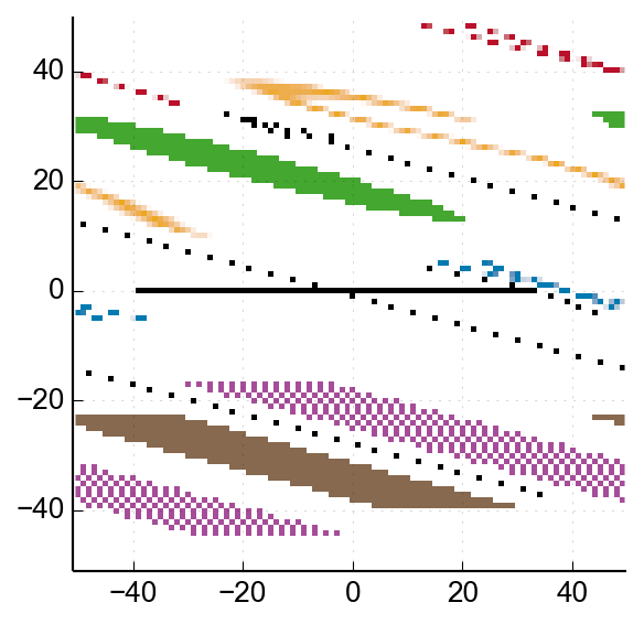
The first skew is so extreme that most of our image has wrapped around at least once, and that throws everything else off. Let's take a look at our skew coefficients for different

Angle units are shown in radians because... because.
As you can see, our vertical skew stays somewhat manageable, but as we get close to a 180° rotation (
Limiting to ±90° or ±45°
There's a straightforward fix, though. A 180° rotation is just flipping the signs of both axes - so let's try again, but this time we flip by 180° first, and then rotate back by -30°:
➔
 ➔
➔
Using an optional pre-rotation of 180°, we only need rotations of ±90° to cover every possible angle. This makes things a bit more fiddly, but it's totally worth it.
If we optionally pre-rotate by ±90° as well (by swapping axes), we can reduce our maximum rotation to ±45°.
Overflow
When rotating an image like this, some of the output pixels can't be correct because their ideal source pixel/co-ordinate is outside the bounds of the image. In general, this can happen (for at least some angle) for anything outside this circle:

But not everything inside this circle is correct in our result either. Here are the operations for a 60° rotation, but this time whenever a pixel wraps around, we shade it in:
➔
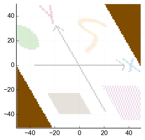 ➔
➔
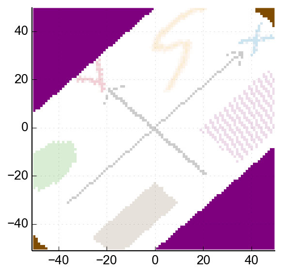 ➔
➔
The problem is really the third step, which produces overflows where we might expect meaningful results:
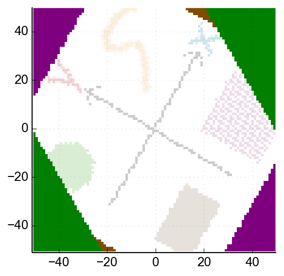
If we allow pre-rotating by 180°, our maximum rotation is ±90° (or ±45° if we allow ±90° pre-rotation). Using the horizontal skew factor

So, if we use 180° pre-rotation, our safe zone is the central diamond. If we include pre-rotations of ±90° as well, we get a bit more, but it's a slightly weird shape (being the intersection of the shallower skew-lines and the circle above). 🤷
Animated examples
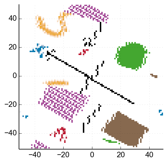
Here's an example using the optional 180° pre-rotation, for various angles:
Each frame in the above animation is a single rotation of the original image, to illustrate the effect of overflow.
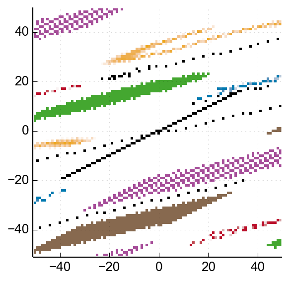
If you instead repeatedly apply a 10° rotation, the cumulative errors are much worse (particularly near the centre):
Ranges for coefficients
In our C++ example code above, we used a 16-bit value int16_t for sinTheta and tanHalfTheta. If we scale it in the obvious way (one sign bit, and 15 fractional bits), this can represent -1 but not +1. We therefore might run into trouble if we try to rotate by something like 89.9°, where
One option is to have more non-fractional bits, by storing the rotation coefficients as int32_t (particularly as we cast to int32_t for the multiplication anyway). Or we could add some extra checking for
As long as we do the same thing for rotate() and inv_rotate(), we won't break invertibility - but if our coefficients wrap around (in some edge-cases) we could get results which don't reflect the rotation we want.
FFT butterfly
We can use this rotation approach to create an entirely reversible fixed-point FFT (or related transforms like MDCT). I'm not going to dive into all the details here - but let's look at just a single radix-2 FFT butterfly:
This is equivalent to multiplying the vector
If we swap the columns around, and apply an extra scaling factor, you get the matrix for a -45° rotation:
So, the radix-2 FFT butterfly can be represented as a rotation, plus a bit of extra fiddling with columns/signs. (There's no complex multiplication here, so we'd just rotate the real/imaginary parts independently.)
Between this, and using this rotation approach for the twiddle-factors, you can hopefully see how we could construct a lossless fixed-point (I)FFT.
Comparison with floating-point FFT
In a floating-point FFT, we avoid the
We can't avoid this factor in fixed-point FFTs (because it's required to be invertible), which means our butterflies take more computation. In addition, the knock-on effects of overflow in one butterfly (which we don't get with floating-point) are hard to intuitively predict. If our signal is close to full-scale, we could end up with results which don't intuitively match the signal.
Conclusion
We've seen how you can rotate a fixed-point complex number in a perfectly reversible way, and used image rotation as an analogy, including the effect of overflow. We briefly sketched out how this enables a fully-invertible fixed-point FFT.
There are some fiddley details if you want to maximise the correctness of the result, but I think the underlying technique (splitting rotation into reversible skew operations) is just really cool.