Smooth Monotonic Interpolation

Geraint Luff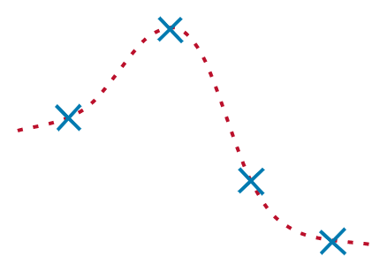

2021-07-09

Producing a smooth, intuitive curve from a set of control points.

Here's something that's not directly audio-related, but comes up a lot in user interfaces for audio tools. The user specifies a set of "control points", and you have to extend those points into a smooth curve mapping one value to another:

This is a friendly interface for the user, useful for things like envelopes (mapping time to amplitude/etc.) or EQs (mapping frequency to amplitude). But in those cases, the curve just being "smooth" isn't enough.

The problem

Let's define a segment as the section of the curve between two adjacent control points.

Here are a couple of things we don't want:

Overshoot is particularly problematic when our control points are at or near 0, and our mapped value (e.g. amplitude) shouldn't really go below 0. But neither of these really look like the curve the user wanted.

Monotonic

The mathematical terms for what we want is a monotonic function between the two points, meaning the gradient of each segment can either be ≥ 0 or ≤ 0, but you can't go both up and down within a segment.

This property means the curve can't have any peaks or dips that aren't exactly at a control point. This is nicely intuitive - when the user wants a peak/dip, they'll tell you exactly where it should be.

Our requirements

So, the curve we want must:

1. pass through all the input points
2. be smooth (continuous gradient)
3. be monotonic within each segment

Smooth interpolation

Let's tackle the first two requirements to start with: smoothly passing through all the input points.

In order to be smooth, the gradient for the end of one segment must match the gradient at the start of the next. A straightforward way to achieve this is to just decide what that gradient should be:

Cubic segments

The segments could be any type of curve, but a common choice is cubic polynomials. With two (control) points and two (chosen) gradients, there is a unique cubic solution:

Let's call our start/end coordinates (x_0, y_0) and (x_1, y_1), and use g_0 and g_1 for our gradients.

We can solve for the cubic coefficients above using some basic calculus and some simultaneous equations - but the solution ends up a bit neater if we define a temporary variable:

t = \frac{x - x_0}{x_1 - x_0} y(t) = a t^3 + b t^2 + c t + d

This gives us the coefficients:

Example code

Here's a C++ class for setting up and evaluating a single cubic segment:

				struct HermiteCubicSegment {
					// How to map x -> t
					double x0, xScale;
					// Cubic coefficients
					double a, b, c, d;

					HermiteCubicSegment(
							double x0, double x1,
							double y0, double y1,
							double g0, double g1) {
						this->x0 = x0;
						xScale = 1/(x1 - x0);

						double m0 = g0*(x1 - x0);
						double m1 = g1*(x1 - x0);
						a = 2*(y0 - y1) + m0 + m1;
						b = 3*(y1 - y0) - 2*m0 - m1;
						c = m0;
						d = y0;
					}
					// We can call this object like: `hermite(x)`
					double operator()(double x) const {
						double t = (x - x0)*xScale;
						return d + t*(c + t*(b + t*a));
					}
				};
			

Choosing gradients

Given a set of points, how do we choose the gradients? There's no single "correct" answer - but this means we can pick a property which feels like it should be true, and see if we can construct a rule to make it true.

Let's say that we have an existing set of points which are following a quadratic curve. Our interpolation should be able to reconstruct this exactly:

This is enough to decide the gradient for each point: we fit a quadratic using the points on either side, and read the gradient from that.

We won't work through the steps here - this is the result:

You'll also need to decide what to do with the first and last points (because either d_k or d_{k-1} is undefined). For simplicity, we're going to give them a gradient of 0.

Smooth (non-monotonic) results

This gives us a smooth interpolated result between our control points:

Other ways to choose gradients

That's just one way to choose the gradient - you could instead take the average of the straight-line slopes on either side:

Or you could weight the straight-line slopes based on the output value (y) difference instead of the input value (x) difference:

Each method will produce a different curve:

Because we choose a single gradient for each point (shared by adjacent segments), the results are always smooth - but we still can end up with overshoot or extra peaks/dips. So let's deal with that!

Making the segments monotonic

It turns out we can make each segment monotonic with two simple constraints:

Flat gradient at peaks/dips

When one of the control points is a local maximum/minimum, we want to make sure the curve produces a minimum/maximum exactly on that point. So let's give those points a gradient of 0:

But this on its own isn't sufficient:

Limiting the gradients

Non-minimum/maximum points can also cause overshoot if their gradients are too steep:

We can handle this by limiting the gradient:

This gradient limit also (conveniently) guarantees that there are no intermediate peaks/dips inside the segment:

So that's all we need to get monotonic cubic segments.

Non-cubic segments

While the flat gradient for peaks/dips is a universal requirement, the gradient limits are specific to the fact that our segments are cubics. The 3x gradient for cubics conveniently also guarantees no intermediate points/dips.

But you might choose a different family of curves for your segments - at which point you'll need a different set of gradient constraints.

Wrapping up

So, to get a smooth curve with monotonic cubic segments:

1. Choose a gradient for each point, with any method you like
2. For all minimum/maximum control points, set their gradient to 0
3. For all other points, apply the 3× limit
4. Generate cubic segments as normal

Results

Here's a look at this algorithm in action:

The curve itself is always smooth, but compared to the non-monotonic version, it doesn't respond quite as evenly when we move the control points - segments will suddenly bump up against one of our two gradient constraints (flat-peaks or the 3× limit).

But it's still neat!

C++ Implementation

Here's a header-only C++ implementation of this algorithm. Just set up the object, and add your points:

						#include "hermite-cubic-curve.h"
						
						HermiteCubicCurve<double> curve;
						
						// if re-using the object
						curve.clear();

						// Add your points
						for (auto point : myPoints) {
							curve.add(point.x, point.y);
						}
						curve.finish();
						
						// Get values out from the curve
						double y = curve.at(x)
					

VST demo

If you're on Mac, you can try out the above class as an interactive demo:

Alright, that's all for now.