Filter-Bank Spectra (and Pitch-Tracking)

Geraint Luff
Signalsmith Audio Ltd.

2026-10-10

Non-uniform spectrum analysis and how it can be useful

This article continues two trains of thought: "multiband and spectral processing are the same thing" from my pitch-shifter talk, and my continuing quest to pull apart a signal with low latency.

What is a spectrum?

Roughly speaking, a spectrum (in audio) is when we pull apart a signal into different frequencies, to gain a perspective on the sound which is closer to how our ears perceive it than just looking at a waveform.

There's a fuzzy boundary between this and multi-band processing. The usual differences are:

resolution: Multi-band processing usually only has a handful of bands, but a spectrum might have hundreds or thousands.
down-sampling: Multi-band processing usually runs at the full input sample-rate, whereas a spectrum is only computed periodically.
resynthesis is optional: The sub-bands of a multi-band split are usually intended to be recombined into a full-band signal. Spectra might be reconstructed, but it's not unusual for a spectrum to be for analysis only (e.g. taking the magnitude for display).

I'm not including how the band frequencies are spaced, because things like the CQT (Constant Q Transform) or Mel-frequency spectrograms can also reasonably be called a "spectrum"

As I said though, there isn't a firm boundary. One of the things I harp on about a lot is that the STFT (Short-Time Fourier Transform) can be used as a band-split, albeit one with complex sub-bands, downsampled results and a very efficient implementation (FFTs).

STFT as a downsampled filter-bank

This is just a quick summary of my explanation from the pitch-shifter talk, but: an STFT is typically viewed (and computed) as a sequence of overlapping blocks, each of which is FFT'd to get a spectrum, and then (after modifying the spectra) IFFT'd and recombined:

For our current task, we won't actually be resynthesising an output stream, but still - we can re-interpret each spectrum as being one sample from each of our (many) complex-valued sub-bands:

What are the windows doing?

If you bash through the equations, the analysis window of our STFT (in the filter-bank interpretation) ends up being the impulse response of a lowpass filter used to band-limit each sub-band before downsampling. If we were generating output, the synthesis window would be the lowpass/bandpass used to upsample back to full-rate.

Bands above f=0 are bandpassed instead, using a (complex) bandpass which is that same lowpass filter, but up-modulated using a complex sinusoid of the appropriate frequency:

A comparison of the window function (solid) which acts as the lowpass for band 0, against the up-modulated kernel which is the complex bandpass for band 5 (dotted, plus dashed imaginary part)

The end result is we have N complex sub-bands, each of which running at a rate reduced by the hop-length L.

Massively parallel time-domain effects

The killer advantage of STFTs is really the downsampling. The sub-bands have a fairly narrow bandwidth, so there simply isn't enough information in each sub-band to need the full rate.

This lowered sample-rate makes a lot of conventional time-domain processors very efficient to do for a ton of sub-bands at once. It even scales really well as you increase the number of bands, since the narrower your sub-bands are (longer STFT blocks) the more you can downsample them (longer STFT interval).

What if we didn't downsample?

Given our galaxy-brain definition above where a spectrum is just a bunch of bandpasses, it's worth comparing this STFT setup against a bunch of full-rate (conventional time-domain) bandpasses. This would have some advantages:

You can choose the centre/bandwidth wherever you want (e.g. log-spaced, perceptual pitch, or resolution of our ears) instead of just linearly-spaced
Wider bands (usually higher ones) can have lower latency / group delay. That means we can have a spectrum which responds faster to higher frequencies, although that precludes straightforward resynthesis.

The disadvantage is that it's much less efficient to compute than STFTs, because we're missing out on the downsampling which gains us so much performance.

Filtering inside sub-bands

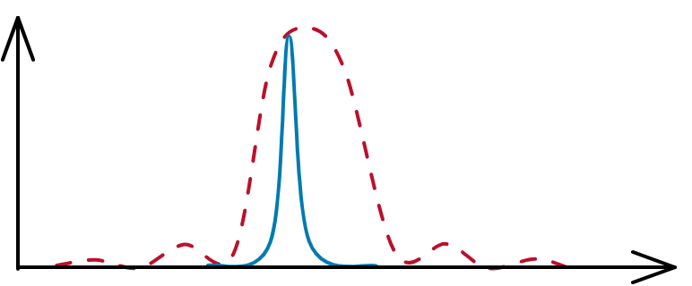
As long as the STFT filters are much wider than the actual bands we want, we can run each bandpass for our spectrum using one of the STFT sub-bands as the input:

We still get to place these bandpasses wherever we like, but they run at the downsampled rate.

STFT block size

The key here is that we're no longer using the STFT to get the narrow sub-bands our spectrum needs. In fact, we actively want sub-bands which are much wider than our spectrum's bandpasses.

There's no single correct answer here, but let's illustrate with a few numbers:

2ms blocks, 0.25ms interval
: That interval means our STFT sub-bands are running at 4kHz, which is 12x downsampled from 48kHz. At 8x overlap, the aliasing from our downsample is somewhere around -100dB, although it depends on the exact window shape.
10ms blocks, 1ms interval
: That interval means our STFT sub-bands are running at 1kHz, 48x downsampled from 48kHz. At 10x overlap, the aliasing from our downsample should be around -130dB with a well-chosen Kaiser window.

I want to reiterate that STFTs are very cheap for the amount of band-splitting they do, but also that the actual bandwidth of the STFT sub-bands doesn't matter as long as it's significantly wider than the actual spectrum bandpasses we want.

So, if you can accept a few ms of latency, and have a decent FFT available, you get to run all your actual spectrum bandpasses at a much lower sample-rate. This gets you a corresponding speedup (e.g. 12x or 48x above) and the more latency (or aliasing) you're willing to accept, the more speedup you get.

Choosing the sub-bands

The bandpasses we want generally won't be centred neatly on one of the STFT sub-bands. We can choose between rounding up or down:

This sometimes works fine, but (especially if these bandpasses might move around!) you might want to interpolate between the two bands, so that there are no odd boundaries when it swaps from using one sub-band to another.

You can even compensate for the amplitude reduction away from the centre of the band, if that dip would be a problem further down the line. That and your choice of window/overlap/etc. will depend a lot on exactly what you're using it for.

Pitch-tracking from a log-spaced spectrum

As an illustration for how this type of spectrum can be useful (beyond just visualising), let's look at pitch-tracking. First, let's think about two closely-related methods:

Autocorrelation and MSD

Autocorrelation and mean-squared-difference (MSD) are methods which choose a wavelength for the signal. For each candidate wavelength, we compare a section of the signal against a delayed copy:

In this diagram, we've taken a windowed segment, and that windowing is applied *before* shifting the copy in time, but you might window after, or only window one. The actual details aren't important here - the key part is the delay.

We can look at either the dot-product of these two segments (autocorrelation) or the difference between them (MSD). But when you work through the equations for these, it's extremely similar to taking a comb-filtered version of the recent input and looking at the energy of a short segment:

Looking at the input's spectrum, and the response of our comb filters, autocorrelation is about picking the comb filter which preserves the maximum amount of energy from the input, by landing the comb's peaks on the input harmonics:

If we change the sign of this comb filter (so it's subtracting the delayed version instead of adding), MSD is about picking the comb filter which preserves the minimum amount of energy, by landing the comb's dips on the input harmonics:

Mathsy detail

Adding the delayed signal gives you autocorrelation, plus some extra energy terms. Subtracting them gives you MSD:

\begin{aligned} & \text{energy of }(A \pm B) \\ &= \int{(A(t) \pm B(t))^2} \\ &= \int{A(t)^2} + \int{B(t)^2} \pm \int{2A(t)B(t)} \\ &= (\text{energy of }A) + (\text{energy of }B) \pm 2\times\text{autocorrelation} \\ \end{aligned}

Let's take the spirit of these two approaches, but calculate them using our spectrum instead:

Combing the spectrum

Above, we sketched the input spectrum out with a linear frequency axis. Let's look at it with a logarithmic scale:

A great thing about the logarithmic frequency scale is that the comb filter's response is exactly the same shape for different frequencies, just with different offsets:

Having the same shape means we can actually use correlation (which can be done very efficiently) to see which position best matches. We also don't need to stick with the equally-weighted peaks which autocorrelation and MSD have.

Octave-down errors

There's a problem though: in the third example above, the comb filter we were evaluating corresponds to a frequency one octave down from what we probably want. However, because all the harmonics were still hit (since they're also harmonics of the lower candidate note) it would score fairly well.

This is a problem which autocorrelation and MSD also struggle with. However, there's another method which doesn't:

Harmonic product spectrum

The harmonic product spectrum (HPS) is an explicitly spectral pitch-tracking algorithm, based on multiplying the spectrum with squished copies of itself. Essentially, the score for a particular candidate note is the product of the energy of its first few harmonics.

Since multiplying values corresponds to adding up their logarithms, we can actually consider HPS as a similar comb-like response, but on \log(\text{energy}):

Taking the logarithm flattens energy peaks a bit, and hugely deepens the dips. We can intuitively see how this could make it more robust to octave-down errors, since having a peak land on a dip where there should be a harmonic can massively reduce the score.

Drawbacks

The flip-side of that is that if a sound doesn't have all the harmonics, then the correct frequency can end up scoring very poorly. HPS fails completely when trying to track a pure sine wave, which I think is a critical flaw.

If the sound does have all the harmonics, HPS is susceptible to octave-up errors. There are some schemes which blend autocorrelation and HPS results, but I think we can do better:

Best of both

So, autocorrelation and HPS can both be considered (or at least approximated) by convolving some kind of "score" curve against a log-spaced spectrum. The difference is whether we take the logarithm of the energy, which flattens spectral peaks and creates huge dips.

Here's the setup that I ended up using:

Take the 8^th root of the spectral energy. This is somewhere between looking at the energy, and looking at its logarithm.
Use a "scoring kernel" which has peaks where harmonics are, and is low in between.
Find the best match for this scoring kernel (which can be done efficiently using FFT convolution).

Here's a sketch of the scoring kernel I used. It only uses the first 10 harmonics (not including DC), and lower ones are weighted more heavily. There's a negative score for energy in-between the harmonics (hoping to avoid octave-up errors), and the width of the peaks relative to their actual frequencies gets wider for higher harmonics, allowing wiggle room for inharmonicity:

If you'd like to give this a whirl, my C++ implementation is up on GitHub.

Use for audio processing

I've mostly mentioned analysis use-cases here, because properly reconstructing the input audio from these spectra is pretty awkward. This makes it a bad fit for "true" spectral-processing effects such as noise-reduction or resonance suppression (although using this analysis to drive a bank of dynamic EQs could work well).

Sometimes you don't need to be exact about reconstruction though, particularly if you're altering the audio anyway. I think this method is strongest when synthesising something which "sounds like" the original input, but transformed enough that listening to the delta (= \text{wet} - \text{dry}) doesn't make sense.

Alright, that's all for now.